ESSC2020 | Climate System Dynamics

Due: 28/9/2021                                                                                                              Total Points: 30

Please give all final numerical answers with no more than three significant figures, but always keep one or two extra significant figures during intermediate steps so you don t lose the precision.

Useful constants:

Solar constant (average):                     S₀ = 1367 W m²

Stefan-Boltzmann constant:               ? = 5.670�10⁸ W m² K⁴

Wien s displacement constant:           ? = 2.898�10³ m K

1. Stellar Spectrum and Planetary Energy Balance (15 points): Below shows the measured electromagnetic spectrum of the star Proxima Centauri, the closest star to the Sun. The measured spectrum can be quite well fitted by a theoretical blackbody spectrum.

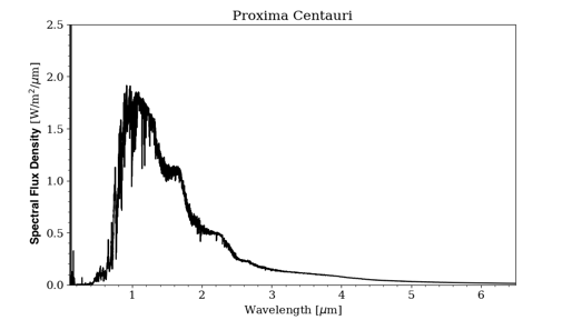
• What approximately is the peak wavelength of the spectrum? (Please note that to find the peak of a spectrum, you should consider the best-fit, smoothed spectrum, and discard the noises.) (1 point)

• What type of radiation does this correspond to? (1 point)

• Estimate the effective temperature of this star. (1 point)

• This star has an effective radius of about 1.07�10⁵ km (i.e., ~15% of that of the Sun). Suppose there is a planet 5.5�10⁶ km away from the center of this star. Based on what you calculated in (c), estimate the average radiant flux density reaching the planet (i.e., the �solar� constant of the planet). (3 points)

• Suppose this planet has a planetary albedo of 0.30, and assume that the effective number of atmospheric absorbing layers of this planet, N, can be represented as a linear function of CO₂ concentration (where [CO₂] is in unit of ppm):

Using the results you obtained in earlier parts and using the multilayer model of the atmosphere, estimate the global surface temperature of this planet if the global CO₂ concentration is currently 400 ppm. Is this planet possibly habitable to life? For a planet to be habitable, it is believed that liquid water should exist at the planetary surface. (4 points)

• Now there is a mega-volcanic eruption that increases [CO₂] to 800 ppm. Calculate the resulting climate sensitivity (?T_s) using the multilayer model and any information above. (2 points)

• The actual equilibrium climate sensitivity finally observed following the volcanic eruption is about +2.8�C. How different is it from what you found in (f)? Explain the difference, and suggest two mechanisms in relation to the variables in the simple climate model that might have contributed to the difference. (3 points)

• Runaway Greenhouse Effect (5 points): The Venusian atmosphere is composed of more than 95% CO₂, with a surface atmospheric pressure more than 90 times that of Earth�s. Scientists believe that around 4 billion years ago, the Venusian atmosphere was more like that of the Earth with liquid water on the surface. The water vapor feedback is believed to have at least in part caused Venus to evolve into today�s �hellish� state in a process known as �runaway greenhouse effect�. The strength of water vapor feedback increases exponentially with temperature because of the Clausius-Clapeyron relation. Suppose the feedback factor f associated with water vapor can be represented as an exponential function of surface temperature T_s (in K):

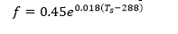
• What should the value of f approximately be for the runaway greenhouse effect to start occurring? Estimate the corresponding temperature (in �C) at which this begins to occur. (2 points)

• Describe and explain the sequence of events that might have occurred on Venus after the runaway greenhouse effect kicks in. Focus on what happened to T_s. (2 points)

• Explain why this runaway greenhouse effect is unlikely to occur on Earth in at least the next few decades. (1 point)

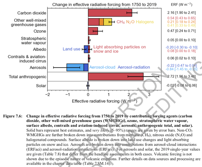
• Radiative Forcing of Aerosols and Clouds (10 points): Next page shows the change in radiative forcing of different climate drivers in year 2019 compared to year 1750 as summarized by the IPCC Sixth Assessment Report (Working Group 1, Chapter 7, Figure 7.6) in 2021.

• What is the total mean radiative forcing from aerosols, including both aerosol-cloud interactions and aerosol-radiation interactions, in year 2019 relative to 1750? Make sure you get the sign correct. Which aerosol interaction is more uncertain in terms of its radiative forcing effect? (2 points)

• Using the �leaky greenhouse� model of atmosphere, estimate the change in planetary albedo (?_p) associated with the radiative forcing coming from aerosols and clouds as you found in part (a), assuming that all other variables in the model remain unchanged (i.e., before the whole climate system adjusts to a new equilibrium, as is usually assumed in the definition of radiative forcing). (2 points)

• Climate feedback due to enhanced aerosols and clouds in the atmosphere alone may lead to a feedback factor of f = �0.06. Explain the physical mechanism behind the sign of f. Calculate the �initial� (without feedbacks) and �final� (with feedbacks) climate sensitivity (?T_s) arising from aerosols (including both interactions), if only aerosol and cloud feedbacks are included in the earth system (i.e., there are no other feedback mechanisms). Assume an initial climate sensitivity parameter of ?₀ = 0.27 �C (W m^�2) ^�1. Make sure you include the correct sign for ?T_s. (3 points)

• The total climate sensitivity in response to the total anthropogenic radiative forcing in year 2019 relative to 1750 is about +1.27�C (AR6 WG1 Ch.7 Figure 7.7). Estimate the overall feedback factor f of the climate system. Please suggest at least two feedback mechanisms associated with well-mixed greenhouse gases that can in part explain the overall sign of f. (3 points)