Chapter 3 Case Problem 4: ROSEY'S ROSES

You are to create a financial analysis for Rosey' s Roses as of December 31, 2022,  and December  31, 2023. Following the Chapter 3 examples,use  the  student file ch3-07.xls  to create a vertical analysis of the balance sheet and income statement as of December  31, 2022,  and December 31,  2023-as well as a horizontal  analysis   of  both  the  income  statement  and  balance  sheet  comparing December   31,  2022,  with  December  31,   2023.  Place  the  vertical  analysis in columns  D and  G on the income  statement labeled o/o   of Sales in cells DS  and GS.  Place  the vertical  analysis in columns D and G on the balance sheet labeled %  of  Assets  in  cells  DS   and  GS.   Place  the  horizontal  analysis  in  column  l labeled  % Change  in cell IS for both the income statement and balance  sheet.

Also  create  a pie  chart  of expenses  for the year  ended  December 31, 2023, formatted in a manner similar  to your chapter  work;  a column  chart  of expense for the years  ended  December 31, 2022,  and December  31,  2023,  formatted in a manner  similar  to your  chapter  work;  and  a ratio  analysis   as  of  December   31 2023.  Note:  You will have to use Excel's  help  feature  to  crea~e the  colurn~ chart, because the columns are not  adjacent  to  one  another   as  in  the  chapter example. Use whatever chart layout you prefer.

Save the workbook as ch3-07_student_name   (replacing   student_name   With your name). Print  all  worksheets  in  Value  view,  with   your   name   and  date printed in the lower left footer and the file name in the lower  right  footer.                                                                                 

2   Navigate ~e  Open window to the location of this  text's student  files. (The location would be wherever you saved  the downloaded  student files from Cengage or from your computer  lab's  server.)

3   Double-click  the file ch3-01,  which should be located   in  a Ch 03 folder.   (You may have to click Enable Editing before you begin.)

4   Click the Income Statement tab if it is  not already  active.

5   Right-click  column C and click Insert to insert  a new column.

6   Click cell C4 and type % as a label to the new column.

7   Click cell CS and type the formula =BS/$B$S;  then press [Enter]. (Note: use an absolute reference in the denominator so you can fill down the formula later.)

8 Click cell CS again and reformat the cell by clicking the % tool in the Number group of the Home tab.

9   Resize column C to reveal the value in  cell C5.

10  Fill down the formula in C5 to C 16 by dragging the handle in the lower right corner of cell C5 to Cl6.  (Note:  this  will also copy down the formatting from cell C5, removing border formats that you can fix later.)

11  Eliminate the formula from cell C8 by clicking the cell and pressing

[Delete],  then [Enter].

12  Add appropriate border formats to cells C6,  Cl3,  and Cl6.

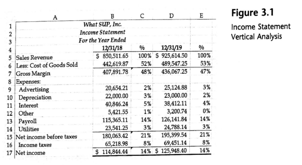
13 Repeat Steps 6 to 11  in column E,  substituting  E for C in all column references.  Substitute D for B in the formulas.  Your worksheet should look like Figure  3 .1.

14  Click File again and then click Save As.  (This preserves your original student and provides a unique name for your file.)

3    Click cell 04  and type % Change  as a label to the column.

4   Format cell 04  bold, center, bottom align, and with a bottom border.

5    Click ceJl 05 and type the formula =(C5-BS)/BS; then press [Enter].

6   Format cell 05  as Percent Style by clicking cell OS and selecting the Percent  Style tool on the Number group on the Home tab.

7    Use the fill-down procedure to copy the formula from 05  to 017.

8    Delete the formula in cell 08.

9   Format cells 06  and D 14 with a bottom border.

10   Format cell 017  with a top and double bottom border.

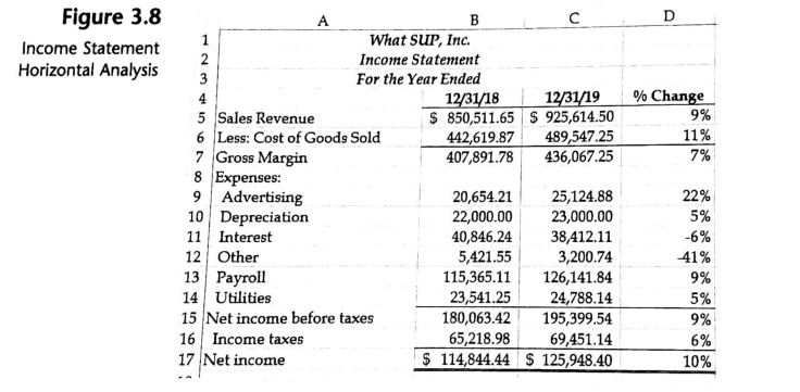
11   Resize column D to 96 pixels. Your completed  income  statement with horizontal  analysis should look like Figure  3.8.

12   Click File and then click Save As. (Again, this preserves the original file by giving a unique name to your file.)

13   Change the file name to include a reference to your horizontal analysis, and then add your name to the file name using the underscore key as before. In this example, the file will be saved as

ch3-01_Horizontal_Analysis_student_name (replace student_name with your name). Save your file to a location from which it can be retrieved later.

14   Switch to a Page Layout view. Place your name in the left section of the footer. Note that the file name is already in the right section of the footer.

15   Switch back to a Normal view.

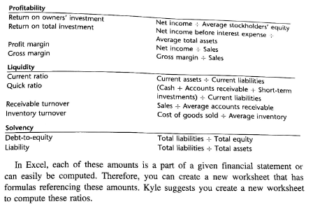
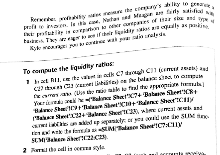
To calculate the first financial ratio on a new worksheet (refer to preceding ratio table for the  return on owners' investment  formula):

1     Right-click the Income Statement tab of your workbook and click Insert ...;  then click Worksheet  and then OK to insert a new worksheet.

2    Double-click the Sheetl  tab and rename the worksheet Ratio  Analysis.

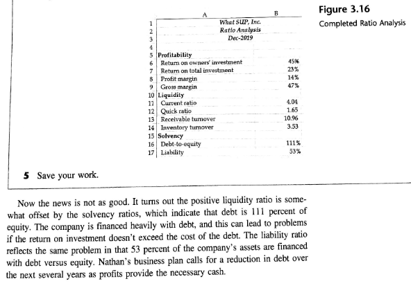
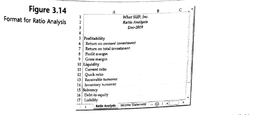
3    Format the Ratio Analysis worksheet like Figure 3.14 with a heading and listing of ratios as shown. To center and merge the title, select the range of cells Al:Bl  and then click the Merge and Center button from the Alignment  group on the Home tab of the Ribbon.  Repeat these steps for the ranges A2:B2  and A3:B3.

4    Click in cell B6 and type the following  ='Income  Statement'!C17/ (('Balance Sheet'!B26+ 'Balance  Sheet'!B27 + 'Balance Sheet'!C26+'Balance Sheet'!C27)/2) to compute return on owners'  investment.

5    Alternatively,   you could  utilize  multiple  worksheet  referencing. Type  = in cell B6, then  activate  the income  statement  worksheet  and click  cell Cl 7.

6    Type/((   (the forward  slash and two left parentheses,  which determine the all-important  order  of calculation).

7   Activate  the balance  sheet worksheet  and click cell B26.

8   Type  +,  then click cell C26.

9   Type  +,  then click cell B27.

1 O     Type  +, then  click cell C27.

11   Type )/2) to end the summation of equity accounts and divide the result by 2 to derive an average.

12   Press [Enter] to end your formula.

13   Format cell 86 in a percent style.

Tr o u b I e ?  If you choose to type the formula as written here and forget an apostrophe or exclamation point or misspell a word,  then Excel will give you an error message  and you'll have to debug your  formula.  Also, if you don't have the correct number of parentheses, Excel will give you an error message.  Note that when you edit the formula, Excel changes the color of each set of parentheses so that you can clearly see which is which. Also be careful when typing formulas to use the apostrophe and not the accent key to create formulas.  The apostrophe key is usually located next to the Enter key on your keyboard, and the accent key is usually located above the Tab key.

'.'The point-and-click method of cell referencing  on multiple  worksheets  is  sure easier than typing the references  themselves,"  you comment. "Otherwise I would have  to type all of those  apostrophes  and exclamation  points.  With  my typing skills,  I would Probably forget one of them and create an error in the formula." Good point,  Kyle says. "Let's finish  the profitability  ratios next."

3  Use the values at cells B 17 and C 17 on the balance  sheet to add total assets, and then divide the result by 2 to obtain average total assets.

4    Once your formula  is typed,  press  [Enter]  to compute  the ratio.  Your formula  should look like this:  =('Income Statement'!C17+'1ncome Statement'!Cll)/(('Balance Sheet'!B17+'Balance  Sheet'!C17)/2). Be careful to use the correct  parentheses.

5   Format the cell in percent style.

6    In cell BB,  use the values at cells C 17 and CS on the income  statement to compute the profit margin. (Use the ratio table to enter the appropriate formula.) Your formula should look like this: ='Income Statement'!Cl 7/'IncomeStatement'!CS.

7  Format  the cell in percent style.

8    In cell B9, use the values  at cells C7 and C5 on the income statement to compute  the gross margin. (Use the ratio table to enter the appropriate fomula.) Your formula  should  look like this:  = 'Income Statement'!C7/ 'Income Statement'!CS.

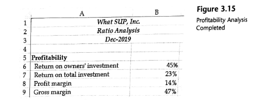
9  Format the cell in percent style. Your window should look like Figure 3.15.

10   Click File then click Save As.

11      Change the file name to include a reference to ratios, and then add your name to the file name using the underscore  key as before.  In this example,  the file will be saved as ch3-0 l_Ratios_student_name (replace student_name with your name).  Be sure to save your file to a safe location.