Demand Estimation
Demand estimation is a method involving estimations of the demand amount of goods or services. The estimations are for a defined timeline and help with pricing. The demand estimations can be computed from a regression equation. Demand estimation provides the market operators with statistical information on the possible future behavior of the market.
Computations of Elasticity
If the maker of a leading brand of low-calorie microwavable food has a demand function of QD = - 5200 – 42P + 20C + 5.2(I) + 0.20(A) + 0.25(M)
(2) (17.5) (6.2) (2.5) (0.09) (0.21) R2 = 0.55 n = 26 F = 4.88 where (P) is price of the product, (A) is the advertising expenditure, and (C) is the price of leading competitor’s product. (I) is the per capita income in the area, and (M) the number of microwave ovens sold in the area. Assuming the following values for the independent variables:
QD = Quantity demanded
P (in cents) = Price of the product = 500
C (in cents) = Price of leading competitor’s product = 600
I (in dollars) = Monthly average income in the area = 5,500
A (in dollars) = Monthly advertising expenditures = 10,000
M = Number of microwave ovens sold in the area = 5,000
The elasticities for each independent variable when P = 500, C = 600, I = 5500, A = 10000 and M = 5000, using regression equation, will be
- QD = -5200 – (42x500) + (20x600) + (5.2x5500) + (0.2x10000) + (0.25x5000)
Quantity demanded will be 17650 units
- Price elasticity = PEoD = (% Change in Quantity Demanded) / (% Change in Price)
=( p/q)x(∂q/∂p)= p/q x -42= (500/17650) x (-42)= -1.19
Therefore, the price elasticity will be -1.19
- Competitor’s (cross) elasticity, from the regression equation, 20c/Qd
= (20 x 600 / 17650)
= 0.68
Therefore, competitor’s elasticity will be 0.68
- Income Elasticity, from the regression equation, 5.2 (I)/ Qd
= (5.2 x 5500) / 17650
= 1.62
Therefore, income elasticity will be 1.62
- Advertising Elasticity, from the regression equation, 0.2(A)/ Qd
= (0.20 x 10000) / 17650
= 0.11
Therefore, advertising elasticity will be 0.11.
- Per capita income elasticity, from the regression equation, 0.25M/Qd
= (0.25x 5000)/17650
=0.07
Therefore, per capita income elasticity will be 0.07
Implications of Computed Elasticity
The computed elasticities have different implications to the business in terms of short-term and long-term pricing strategies. A price elasticity of -1.19 implies a 1% raise in product of price, and a similar decline of 1.19% in the quantity of goods demanded. The demand of the good is elastic since the price has an inverse relationship with the quantity. The price increase may discourage customers from purchasing goods lowering the demand. The competitor’s price elasticity is 0.68 implies that if the price of related good (competitor’s) is increased by 1%, the demand of the product will increase by 0.68. The good is inelastic to price of the competitor’s good; therefore, the competitors’ pricing will not affect sales. An income elasticity of 1.2 means an increase of 1% in the average income will enhance the demand of good by 1.62%. The good is elastic and a rise in price can be considered in case of a raise in average income.
An advertisement elasticity of 0.11 implies that an increase in advertising costs will raise the demand of good by 0.11%. The good is inelastic to advertising, therefore, increase in advertising effort will not automatically allow the company to increase price since it may discourage customers from making purchases. Per capita income elasticity is 0.07, indicating microwave ovens in the region. An increase of 1% in the number of ovens increases the quality demanded by 0.07, which is an insignificant amount. The demand is inelastic and a strategy in pricing can ignore the aspect of per capita income elasticity. Accordingly, quantity demanded is responsive to price of good and earnings of consumers but rather unresponsive to the price of the competitor. Quantity demanded is insensitive to advertising and the number of microwaves in the region.
Recommendation for cutting Market share to Increase Market Share
A reduction in price of a good will increase the amount demanded because the price elasticity is negative and less than -1 or has an inverse relationship to demand. In addition, unity is a bit less over elasticity, and income is maximized when degree of elasticity is 1. In this light, price cut will increase demand, and ultimately, a net increase in sales as elasticity is pushed towards unity (Ferreira, Sara, & José 60). The organization should therefore, cut the price in order to increase the market share and total income derived. The equation below explains the scenario.
Total revenue = price x Quantity
∂total revenue/∂P = Q (∂P/∂P) + P (∂Q/∂P)
= 1+ Elasticity
If E< -1 (elasticity good), then ∂TR/∂P > 0 implying that a decrease in price will lead to a raise in revenue and demand.
Demand and Supply Curve
Assuming thatall the factors affecting demand in this model remain the same, but that the price has changed, and the price changes are 100, 200, 300, 400, 500, 600 cents. The demand curve for the firm will be as follows:
When all factors are held constant, and the demand equation is substituted,
Quantity = (-5200) – (42xP) + (20x600) + (5.2x5500) + (0.2x10000) + (0.25x5000)
Quantity = 38650 - 42P
Price = 38650/42 - Q/42
Figure 1
Demand Schedule in cents against quantity in kilograms
Price (Cents) Quantity
| 100 | 34450 |
| 200 | 30250 |
| 300 | 26050 |
| 400 | 21850 |
| 500 | 17650 |
| 600 | 13450 |
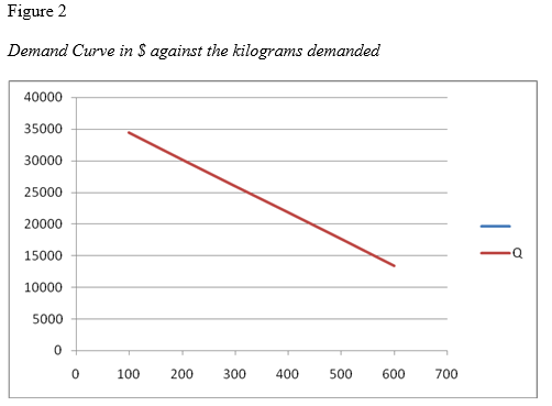
The X-axis is Price in Cents while the Y-axis is Quantity demanded
The corresponding supply curve using the supply function Q = 5200 + 45P with the same prices will be as follows:
Quantity demanded = 5200 + 45P, therefore, Price will be
P = -5200/45 + Q/45
Figure 3
Supply Schedule in $ against kilograms supplied
Price Quantity
| 100 | 9700 |
| 200 | 14200 |
| 300 | 18700 |
| 400 | 23200 |
| 500 | 27700 |
| 600 | 32200 |
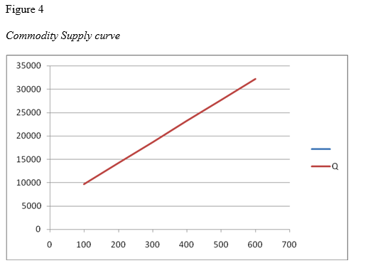
The X-axis denotes the Price in Cents while the Y-axis denotes Quantity demanded
The equilibrium price and quantity will be as follows: at equilibrium price, the quantity demanded and supplied intersect at a point, therefore, the demand function is equal to the supply equation. Substituting the values,
5200 + 45P= 38650-42P
-87P = -33450
P = 384.48
Q = 38650- (42x384.48)
= 22501
Therefore, at the equilibrium price of 384 cents, quantity demanded (equilibrium quantity) is 22,501 units.
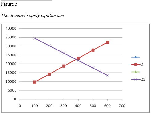
The equilibrium point on the graph above is the intersection point between Q1, which is the demand curve and Q, the supply curve.
Factors That Cause Changes In Demand and Supply
Various factors affect the demand and supply of a good such as consumer income, competitor’s price, and price of related goods. Market conditions in both the short term and long run may affect the demand and supply of a product as well. An increase in consumer income or price of related goods will increase the demand of microwave ovens. An increase in price and change in consumer preference will reduce the quantity demanded. Supply of the good can be altered by the change in number of suppliers of related products, technological innovations, cost of raw materials and labor (DeCicca, Philip, and Don Kenkel 1098). The factors have a direct impact on the production cost. An increase in production cost leads to a price increase in goods demanded, thereby, reducing the amount of supply.
Factors Affecting Shifts in Demand and Supply Curve
A raise in consumer income and a decrease in price of a related good will result in a shift to the right of the demand curve. A rise in the population and preference for the good will also cause a right shift in the demand curve. A reduction in consumer income, economic recession, increase in competitor’s price, and decrease in preference for the good will cause a leftward shift in the demand curve (Dikgang, Johane, Anthony, and Martine 3341). An increase in technological innovations and advances in food manufacturing, availability of cheap labor, reduced cost of raw materials, and raise in tax-cuts will cause a rightward shift to the supply curve.
Increase in the cost of production, increase in the costs of labor and raw materials, and a raise in taxes will cause a leftward shift in the supply curve. In conclusion, demand estimation helps in pricing strategy and monitoring of market conditions. Accurate estimations help an organization in planning and budgeting for production and selling functions.
Works Cited
DeCicca, Philip, and Don Kenkel. "Synthesizing Econometric Evidence: The Case of Demand Elasticity Estimates." Risk Analysis 35.6 (2015): 1073-1085.
Dikgang, Johane, Anthony Leiman, and Martine Visser. "Elasticity of Demand, Price And Time: Lessons From South Africa's Plastic-Bag Levy."Applied Economics 44.26 (2012): 3339-3342.
Ferreira, Sara, and José da Silva Costa. "Price Elasticity of Travel Demand: The Case of the A28 Motorway, A Public-Private Partnership in Portugal."International Journal of Transport Economics 42.3 (2015).
Ismail, Rahmah, et al. "Labour Demand Elasticity and Manpower Requirement in the Malaysian Service Sector." International Review of Business Research Papers 11.2 (2015).